I describe a workflow that uses Docker and Luigi to create fully transparent and reproducible data analyses. End users can repeat the original calculations to produce all the final tables and figures starting from the original raw data. End users (and the author, at a later date) can easily make isolated changes to the middle of the pipeline and know that their changes propagate to all the other steps in the process. I demonstrate this workflow by applying it to the study of drinking water contamination in Mexico.

You can find my full code in this project’s GitHub Repo, and its Docker image in the project’s DockerHub Repo. For a detailed description of how I made the maps that went into this work, see my Geopandas Cookbook. As of Aug 29, 2019, this analysis is now published in Science of the Total Environment, with myself as corresponding author.

The motivation

Historically, my data science workflows were built in Jupyter notebooks. pd.read_csv() imported raw data in the first cell, and df.to_csv() or plt.savefig() exported the final results in the last cell. I carefully commented the intermediate steps so that my thought process was clear, and I saved the notebook for posterity.

A few weeks later, though, I would always run into the same problem. I’d revisit the project and want to change a detail in one of the figures. Or maybe I’d have a new question about one of the intermediate dataframes. Either way, if I wanted to observe or change anything in the middle of the pipeline I’d have to run the whole notebook again just to get to the middle. More often than not, those changes would also break the code written in the last cells. Even more commonly, I would discover that right in the middle of the notebook I’d imported more data that was generated elsewhere and whose exact origin and nature were undocumented. What was that data, again? Which version did I use? Code written a few months ago might as well have been written by someone else, as they say, and I frequently discovered just how difficult it is to keep track of information flows in and out of notebooks. This was not code that could be used in production.

What I love about software engineering is that there are really good tools to address this universal problem, which plagues science in general and data science in particular. Researchers are more and more frequently using Git to track versions, Docker to package their compute environments, and workflow managements systems like Airflow or Luigi to manage the dependencies between all the tasks in their analyses. I’ve applied all these tools to a real-world research project. Let’s take a look at how they work together.

The science

In 2018, the Mexican National Water Commission (CONAGUA) published one of the most comprehensive datasets ever to be collected on the topic of water quality in Mexico. This data included measurements of six trace-element contaminants (arsenic, cadmium, chromium, mercury, lead, and fluoride) in 14,058 water samples from 3,951 sites throughout the country, all collected during 2017.

Water pollution with trace elements, particularly arsenic and fluoride, is a public health problem whose existence is well documented but whose exact scale remains unknown. I dove into this dataset to find out how arsenic and fluoride (As and F) are distributed in the country, and to estimate the health burden associated with continuous exposure to these contaminants. My task required mapping all the sampling sites, visualizing which sites are contaminated, determining the population exposed to that contamination, and estimating the health burden associated with that exposure.

This analysis is be the basis of a paper currently under review, Co-occurrence of arsenic and fluoride in drinking water sources in Mexico: Geographical data visualization.

The tools

Cookiecutter generates structure for your data science project. It creates a good folder structure, and populates it with some necessities like .gitignore files, a license statement, and a few files for packages that generate documentation automatically (though I don’t use that functionality in this project). It also has the most sensible project structure I have found, one that clearly separates your raw data, generated data, python scripts, reports, etc.

Moreover, peole have made versions of this package for different niche applications, and I found a really useful one for Luigi workflows: Cookiecutter Data Science with Luigi. The nice thing about this version is that it comes with:

1. A script final.py with a Luigi task FinalTask that you will populate with dependencies to all the other tasks in your project.
2. A GNU Make Makefile with a couple of commands that check your programming environment, clean up data, or execute FinalTask.

The upshot of this arrangement is that, once everything is in place and you’re in the root folder of your Docker container, you can type make data into the terminal and Luigi will run all the tasks that haven’t been run yet. One command is all you need to re-create any parts that are missing, or even the entire project. (There’s also make data_clean to remove all the stuff you just created, and both can be customized).

I adapted the Cookiecutter folder structure to include a folder for Docker operations and to remove stuff that I wasn’t using, and wound up with this:

├── LICENSE
├── Makefile           <- Makefile with commands like `make data` or `make train`
├── README.md          <- The top-level README for developers using this project.
├── data
│   ├── external       <- Data from third party sources (zipped maps of Mexico, INEGI town data)
│   ├── interim        <- Intermediate data that has been transformed. Includes unzipped maps.
│   ├── processed      <- The final, canonical data sets for mapping.
│   └── raw            <- The original, immutable CONAGUA data.
│
├── docker             <- Dockerfile and requirements.txt
│        
├── notebooks          <- Jupyter notebooks that explore the processed datasets.
│
├── reports            <- Generated analysis
│   └── figures        <- Figures generated by this analysis
│
├── src                <- Source code for use in this project.
│   ├── __init__.py    <- Makes src a Python module
│   │
│   ├── data_tasks     <- Scripts to unzip or generate data
│   │
│   └── visualization  <- Scripts that generate maps
│
└── test_environment.py <- Checks current python version.  For use with Make.

For more about the usefulness of Cookiecutter and how to think about organizing your data science project, check out Cookiecutter Data Science — Organize your Projects — Atom and Jupyter.

Docker builds lightweight containers (similar to virtual machines) that contain everything you need to run your analysis, from the operating system to all the python packages that your process depends on. For a good introduction to Docker, check out How Docker Can Help You Become A More Effective Data Scientist.

In addition to the standard folder structure created with Cookiecutter, this project’s GitHub repo includes a docker folder with nothing but a Dockerfile and requirements.txt. These two files are all you need locally to build a Docker image, instantiate it into a Docker container, and fully recreate my programming environment. Alternatively, if you don’t want to wait for Docker to build the image from these instructions, you can pull the image straight from this project’s DockerHub repo.

To test out my system, I cloned the GitHub repo to an AWS Sagemaker instance, pulled the Docker image from DockerHub, instantiated and entered a new container from that image, and typed make data into the terminal. After a few minutes, the whole analysis and all its figures had been reproduced on-site.

The most useful source of Docker commands is not the official documentation, but actually this Docker cheat sheet that links to it. This presentation (and its slides) from ChiPy 2017 has several good examples, though note that some of the Dockerfile syntax has changed since it was published. This presentation (and its repo) from PyData LA 2018 has updated syntax and a much clearer walk-through for beginners.

Luigi is one of the few workflow management tools that are built entirely in Python (as opposed to having their own language, like GNU Make does). Luigi allows you to design modular, atomic tasks with clear dependencies. The idea is that all the steps in your project—from unzipping files to training models and making figures—should be written out as a separate task with known inputs and outputs. Luigi tasks can be swapped out for upgrades or repairs like fuses in a fusebox, which vastly increases the ability of future you to come back to an old project and change a little detail in the middle of the workflow.

When I needed to update my figure legends, for example, I went back to the parent class BaseMap (which inherits from Luigi.Task) and updated the method make_legends(), thus updating the 7 different descendant tasks that created the maps for the paper. I deleted the existing figures so that Luigi would run the task again, and make data promptly made the new figures for me.

For more about project organization and Luigi, check out A Quick Guide to Organizing [Data Science] Projects (updated for 2018) and Why we chose Luigi for our NGS pipelines. For the best introduction to Luigi syntax and motivation, check out this presentation from PyCon 2017 starting at minute 8:25. For a more complex machine learning project built around the same principles, check out this presentation (and repo) from PyData Berlin 2018.

How to set up a Docker work environment

Make the folders

Start out with the structure for the project (and thus for the folder tree). Install Cookiecutter on your machine and make a new GitHub repo, or go to an existing one approach it like a messy closet. Take everything out into a temporary folder, create the new folder tree in your root folder (I’ll call it repo_root), and carefully bring the important contents into the new structure. The main Cookiecutter page walks you through the commands.

If you’re using Cookiecutter Data Science with Luigi like I am, take a moment to familiarize yourself with final.py, the script where you’ll import all the other scripts and add all the other tasks as dependencies. Change the folder structure within src to reflect the broad categories of operations that your project will require.

# repo_root/src/data_tasks/final.py

import luigi

class FinalTask(luigi.Task):
    def requires(self):
        pass

    def output(self):
        pass

    def run(self):
        pass

Make a starting image from a Dockerfile

Make a new folder docker in repo_root, and create a new Dockerfile and an empty requirements.txt. You want to import a Docker image that represents a good minimal starting point to build on. If you want a relatively heavy image with everything you need for a machine learning project, consider one of the images in the Jupyter Docker Stacks. If you have a simple project like mine, consider starting with a more minimal image that has only Python. I used the image Python:3.7.3, which I think is based on some form of Ubuntu. For future projects I’ll choose an image based on a more minimal operating system like Alpine Linux.

# repo_root/docker/Dockerfile

FROM python:3.7.3
LABEL maintainer="Daniel Martin-Alarcon <daniel@martinalarcon.org>"
WORKDIR /app
RUN apt-get update && apt-get install -y python3-pip
COPY requirements.txt .
RUN pip3 install -r requirements.txt && \
    pip3 install jupyter
EXPOSE 8888
VOLUME /app
CMD ["jupyter", "notebook", "--ip=0.0.0.0", "--port=8888", "--no-browser", "--allow-root"]

The order of the elements in the Dockerfile matters, as each line adds a new layer. More immutable elements (like installing pip3) should come first, since Docker can use cached versions of that layer rather than running the operation again. You can even use multistage builds to minimize your image size, as described here. If you’re starting out with a different base image than mine, you’ll probably have to add different commands at this stage. The introductory guides mentioned earlier contain a few different Dockerfiles that work, and How Docker Can Help You Become A More Effective Data Scientist contains a great description of common Dockerfile commands and why you’d want to use them.

As for the commands here, a few notes:

• WORKDIR /app: Creates a new directory and makes it the default.
• COPY requirements.txt .: Copies the file from your local machine to the current working directory (referenced by that lonely dot at the end).
• EXPOSE 8888: Exposes the container port 8888 to the world.
• VOLUME /app: Is really more of a note to the user that external volumes should be mounted to this container directory, if you mount directories at runtime (and we will).
• CMD ["jupyter", "notebook", "--ip=0.0.0.0", "--port=8888", "--no-browser", "--allow-root"]: Is the final command that executes when the container is instantiated. It opens a Jupyter notebook inside the container and connects it to container port 8888 without trying to open a browser (because we never installed a browser).

You’ll know that your Dockerfile works once you can run this command from inside the repo_root/docker folder…

$ docker build -t image_name .

… and get a success message:

Successfully built 32c7086f1e79
Successfully tagged image_name:latest

You should also regularly run docker image ls and docker container ls to keep track of current images and containers.

Instantiate and enter a new container

Once your image is built, it’s time to instantiate it into a container and start working from inside, in our fresh new computing environment. Run this on your local machine:

$ docker run --name container_name -p 9999:8888 -v /path/to/repo_root:/app image_name

This is what the command is doing:

• --name container_name: Assigns a new name to the container you are about to instantiate.
• -p 9999:8888: Connects port 8888 in the container (where Jupyter is!) with port 9999 on your machine.
• -v /path/to/repo_root:/app: Mounts folder repo_root on your computer to folder app in the container. Changes in one will be reflected in the other. More importantly, changes in the container will remain in the local folder after the container is closed or deleted. That’s how our container will export its results to the outside world.

Your terminal should produce output like this:

[I 23:32:22.207 NotebookApp] Writing notebook server cookie secret to /root/.local/share/jupyter/runtime/notebook_cookie_secret
[I 23:32:23.650 NotebookApp] Jupyter-nbGallery enabled!
[I 23:32:23.652 NotebookApp] Serving notebooks from local directory: /app
[I 23:32:23.652 NotebookApp] 0 active kernels
[I 23:32:23.653 NotebookApp] The Jupyter Notebook is running at:
[I 23:32:23.653 NotebookApp] http://0.0.0.0:8888/?token=f93ec866b52666f1aa9e52e45e53da390ff541084c55a529
[I 23:32:23.653 NotebookApp] Use Control-C to stop this server and shut down all kernels (twice to skip confirmation).
[C 23:32:23.655 NotebookApp] 
    
    Copy/paste this URL into your browser when you connect for the first time,
    to login with a token:
        http://0.0.0.0:8888/?token=f93ec866b52666f1aa9e52e45e53da390ff541084c55a529

And if you open your browser to localhost:9999, you should see a Jupyter splash page prompting you for the token that your container just generated.

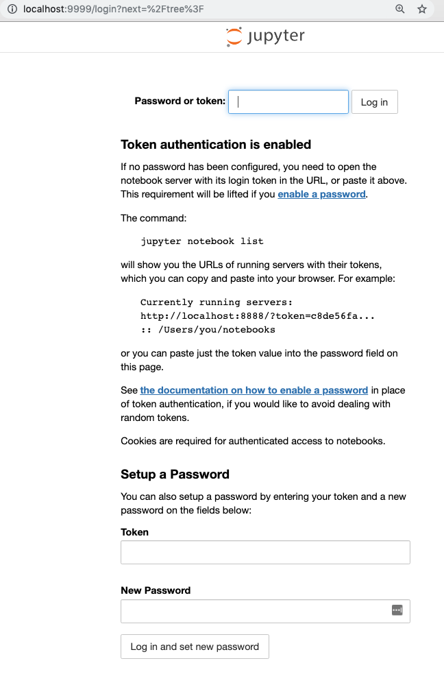
Enter the token (f93ec866b52666f1aa9e52e45e53da390ff541084c55a529) and Log In to see the folder structure inside your container, now accessible through Jupyter.

To run a bash shell inside the container, open a new terminal window on your local computer and run:

$ docker exec -it container_name /bin/bash

Now you should see that the terminal prompt changed, and that you are now inside the container! Check out which programs are installed with pip list, and get ready to start installing more stuff.

Update the image with new packages

From this point, I normally keep three terminal windows open: one running Jupyter inside the container, one running a bash shell to my local machine, one running a bash shell to the container. I sometimes edit the container’s contents from the inside by creating files with make data, and sometimes from the outside by changing the folders that are mounted to the container (in this case, everything in repo_root). If you use VS Code, note that it has useful plugins for seeing currently available images and containers.

As you start working, you’ll figure out what new Python packages you need for your project. After you install them in the container, remember to occasionally export those dependencies to requirements.txt. Do so by running, from inside the container:

$ pip freeze > docker/requirements.txt

Thus the empty file that you created earlier will get replaced with a list of your dependencies. Occasionally shut down your container and rebuild the image with these new dependencies, and definitely do so in the end, to check that your image works.

How to build a Luigi workflow

You’re probably used to designing a linear workflow that goes step-by-step down the page of a Jupyter notebook. In fact, if you’re refactoring an old project then that’s probably how your project is already written up. Your job now is to turn each of those steps into a Luigi task, to organize those tasks into python scripts of similar tasks, and to put those scripts into the overall folder structure that you have in src.

Let’s start with your most common tool, the humble Luigi task.

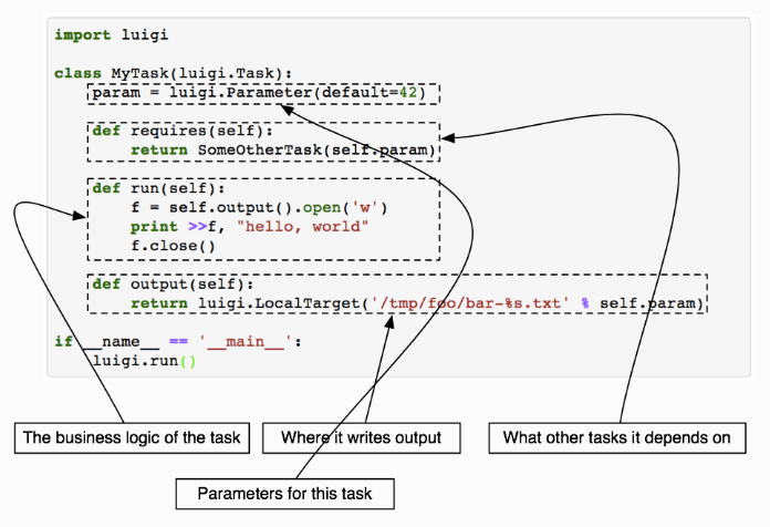
Here’s a task written within our folder structure, which produces a pandas DataFrame and exports it to CSV.

# repo_root/src/data_tasks/getting_started.py

import luigi

class Task3(luigi.Task):
    # Global variables
    output_file = "processed/conclusions.csv"
    
    def requires(self):
        # 
        return [Task1(), Task2()]
        
    def output(self):
        return luigi.LocalTarget(self.output_file)

    def run(self):
        # [Code that makes a pandas DataFrame]

        # The file gets exported to CSV
        df.to_csv(self.output_file)

When a task is executed, Luigi will first check all the dependencies listed in requires(), verify that they’ve been met, and then run all the commands in run(). These commands should produce some sort of result (here conclusions.csv) and write it to a particular place in the folder structure (here data/processed/).

The output() method serves two purposes. First, it allows Luigi to check whether the result has been generated. output() returns a Target object tied to a filename. Target has a single method, exists(), which returns True if there is in fact a file at the declared location. Luigi uses the Target object returned by the output() method to determine whether the task is complete or needs to be re-run. Thus, if you’ve edited the contents of your Task3 above and want to generate a new version of the results, delete conclusions.csv and run make data again.

The second purpose of output() is that it returns the Target object, so that the next task can take it as input. This is how the output of one task becomes the input of the next. If we wanted to access the file produced by Task2 above, we could access its file path as self.input()[1].path. You can see some examples of how tasks are chained here and here.

For simple usage, though, there are only three things to remember about Luigi:

1. run() should generate some file
2. output() should point to that file
3. requires() should list the predecessor tasks that produce the pre-requisites for this one.

Also, if you want to run a task without all the others, you can invoke it individually after cd’ing into the data folder:

$ PYTHONPATH='../src/data_tasks' python -m luigi --module [SCRIPT_NAME] [TASK_NAME] --local-scheduler

A note about folder context: The Makefile is designed such that tasks are run from the data folder. Thus, you should write your tasks as if they will always be run from inside data. That’s why, in order to place the output at repo_root/data/processed/, I only have to specify processed/.

How this project uses Luigi workflows

I started out with an older version of my workflow, designed in Jupyter. I removed all those files from my folder structure and added their operations back in one-by-one, as Luigi Tasks written out in separate python scripts. I strove for each task to represent a single operation with the data, and used class inheritance to keep the code as non-redundant as possible. I then called all the tasks I’d written as requirements in FinalTask, which wound up looking like this:

import luigi

from sys import path
path.insert(0, '/app/src/data_tasks')
path.insert(0, '/app/src/visualization')

from extract_maps import UnzipFiles
from extract_samples import CleanAndExportSamples
from bubbles import AllSitesMap
from bubbles import AllContaminantsMap
from bubbles import EachContaminantMaps
from bubbles import ArsenicAndFluorideMap
from bubbles import GeologyMaps
from sample_town_interactions import WhichTownsAreNearSites
from aggregate_nearby_sites import AggregateNearbySites
from make_summaries import ArsenicSummary
from make_summaries import FluorideSummary
from chloropleths import ArsenicMap
from chloropleths import FluorideMap

class FinalTask(luigi.Task):
    # Global execution variables. Change here for whole project.
    titles = False # Do figures have titles?
    radius = 5 # Radius for contamination effects
    geo_maps = ['arsenic','fluoride'] # Make geology maps for these contaminants
    zipped_files = ['towns','country','states','municipalities']

    def requires(self):
        yield UnzipFiles(self.zipped_files)
        yield CleanAndExportSamples()
        yield AllSitesMap(self.titles)
        yield AllContaminantsMap(self.titles)
        yield EachContaminantMaps(self.titles)
        yield ArsenicAndFluorideMap(self.titles)
        yield WhichTownsAreNearSites(self.radius)
        yield AggregateNearbySites(self.radius)
        yield ArsenicSummary()
        yield FluorideSummary()
        yield ArsenicMap(self.titles)
        yield FluorideMap(self.titles)
        yield GeologyMaps(contaminants=self.geo_maps, title=self.titles)

    def output(self):
        pass

    def run(self):
        pass

I could also have designed this such that all the tasks were linked with each other and FinalTask required only the penultimate task in that dependency list. I relied on the folder structure heavily, making data flow from folders such as raw and external to interim and processed. I wrote tasks such that they referred to locations this folder structure. An alternative way to do it is to rely more on the wrapper self.input() within each task’s run() to refer to the outputs of upstream tasks. This allows the user to transmit the location of data between tasks without ever hard-coding file paths into intermediate tasks.

Project results

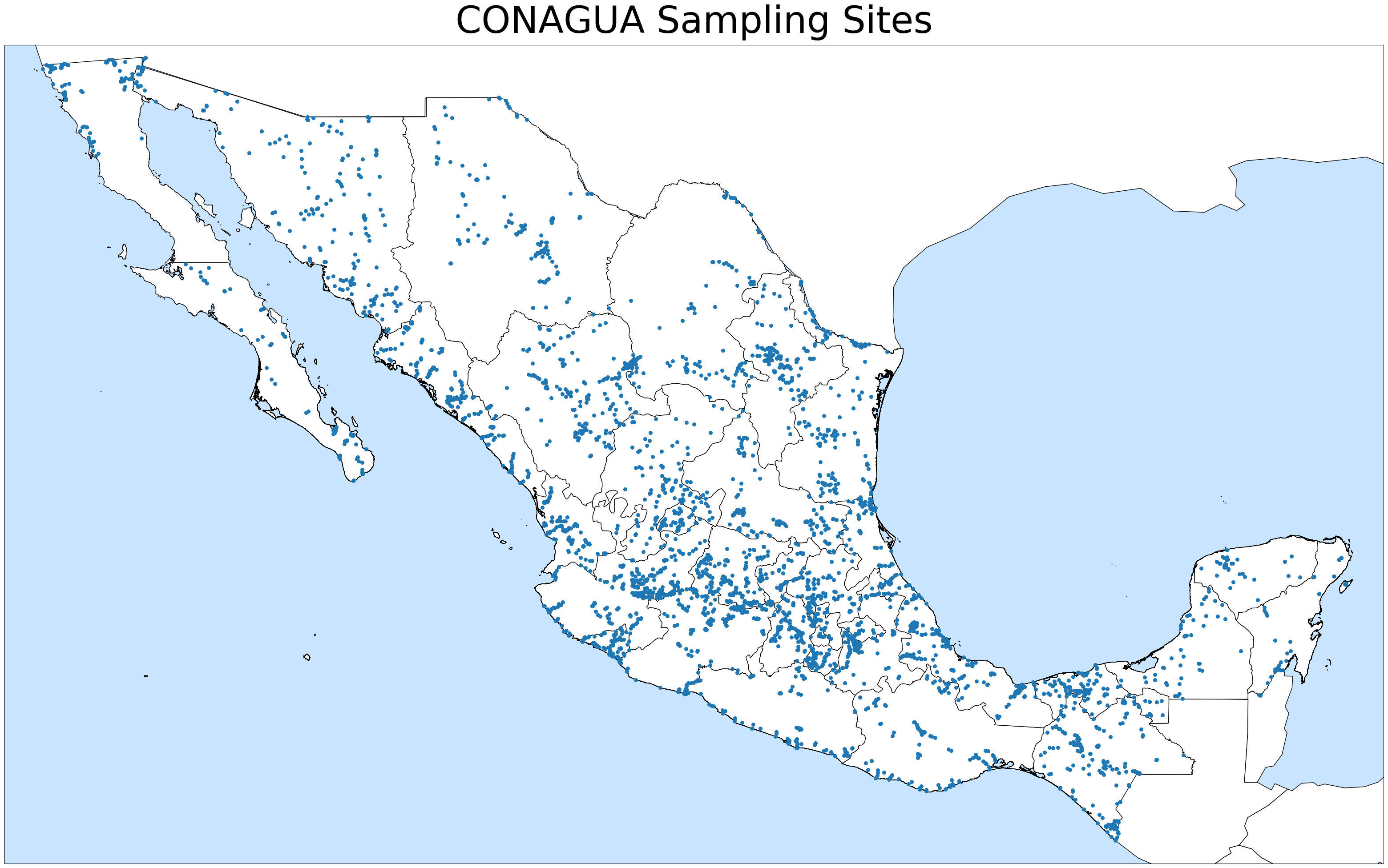
I cross-referenced the 3,951 sampled sites with over 192,000 towns around the country, filtering the latter for proximity to the former. These are the locations of all the sampling sites:

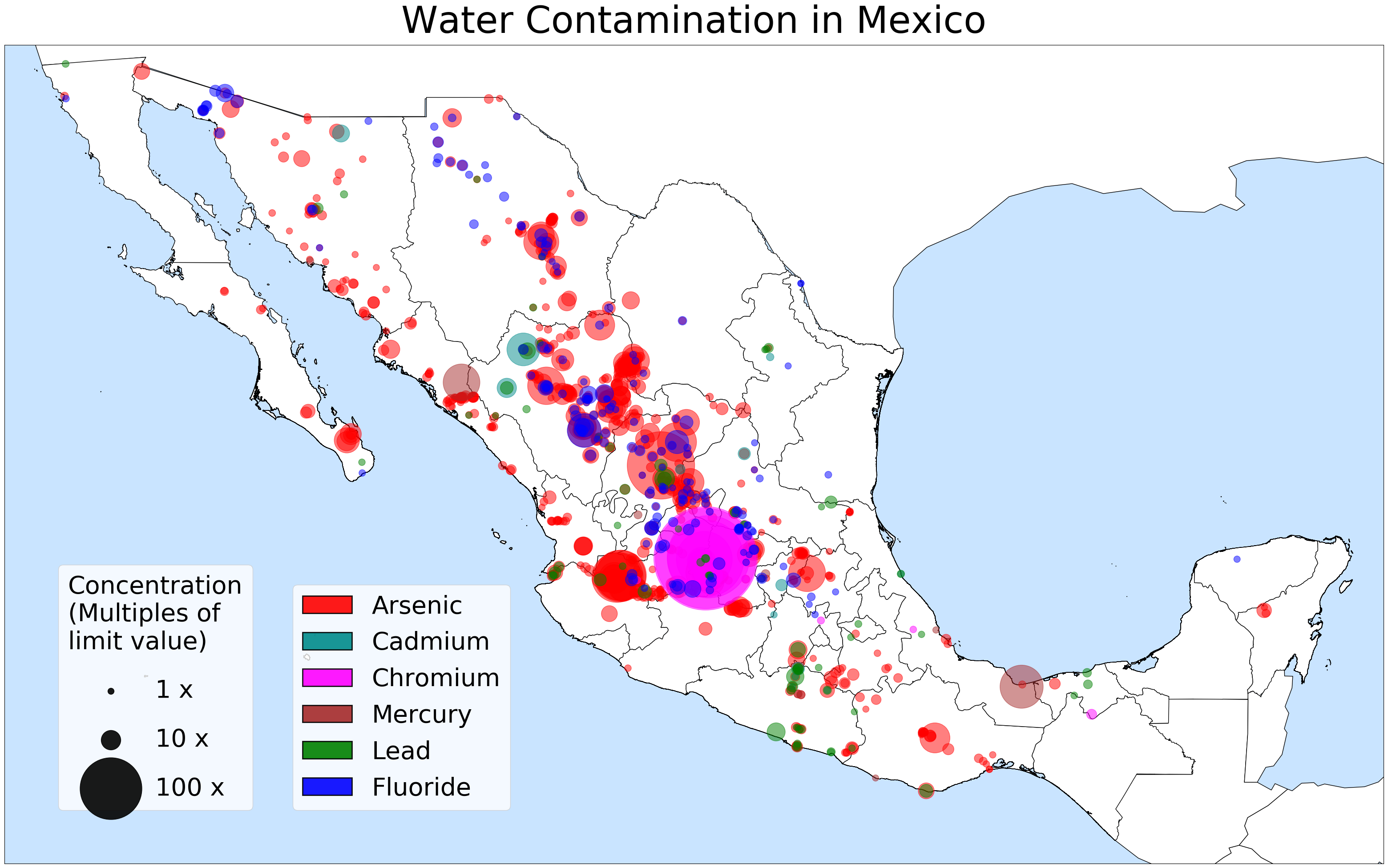
I mapped and plotted the location of six different contaminants wherever they exceeded the healthy limit:

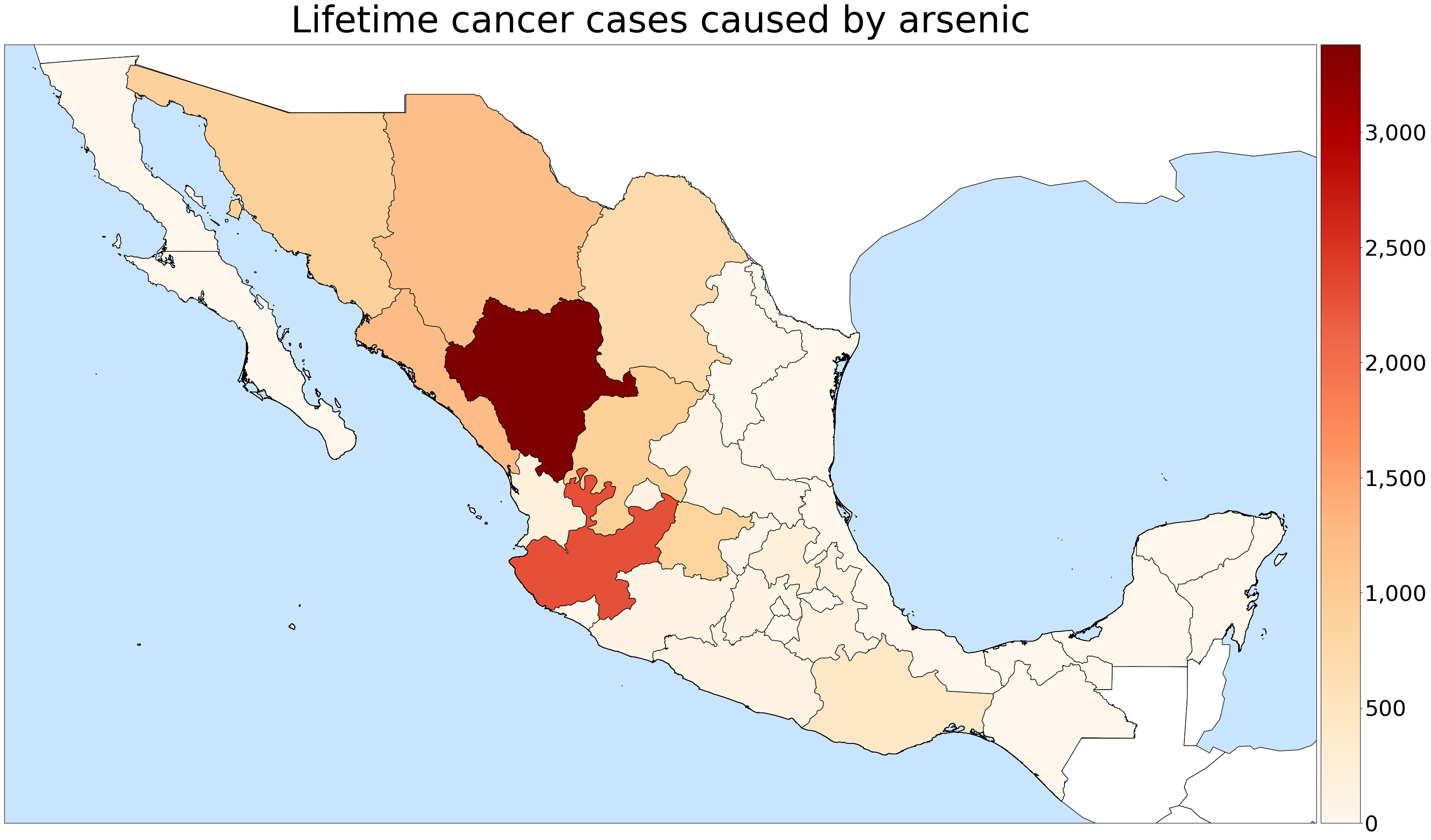
For each town, I assumed that the population was exposed to the average contamination of all the sites within 5 km, and used this to estimate several public health indicators related to arsenic and fluoride contamination. As one salient example, I calculated that chronic arsenic exposure would probably be responsible for an additional 13,000 lifetime cases of cancer in the country, affecting mostly the arid states of Durango and Jalisco.

I estimate that about half (56%) of the Mexican population lives in a town within 5 km of a sampling site, 3.05 million of them are exposed to excessive fluoride, and 8.81 million are exposed to excessive arsenic. The results of this data analysis are currently under peer review, in preparation for publication.

You can find my full code in this project’s GitHub Repo, and its Docker image in the project’s DockerHub Repo.