I combine two very different approaches to time series forecasting, applied to a dataset of air pollution in Beijing. I use Prophet to make an univariate additive regression model, then show that it performs similarly to a shallow neural network made with fast.ai. I devise a plan to give the neural net access to multivariate weather features, both historical data points and feature predictions made with Prophet. I encounter severe data leakage, work through a differential diagnosis, plug the leak, and finally produce an ensemble model with reasonable behavior, if unexpected results.

Smog and weather

Forecasting works best when you have at least a few relevant cycles of feature variation to observe. That’s why I choose to work with the Beijing PM2.5 Data Data Set, a data set of weather and pollution with four years of hourly readings. The dependent variable is 2.5-micron particulate matter, or pm2.5, and there are also six weather features:

# Feature names
feat_name_dict = {
             'pm2.5':'Pollution (pm2.5)',

            'dew_pt':'Dew point',
              'temp':'Temperature',
              'pres':'Pressure',
          'wind_dir':'Wind Direction',
          'wind_spd':'Wind speed',
        'hours_snow':'Cumulative hours of snow',
        'hours_rain':'Cumulative hours of rain'}

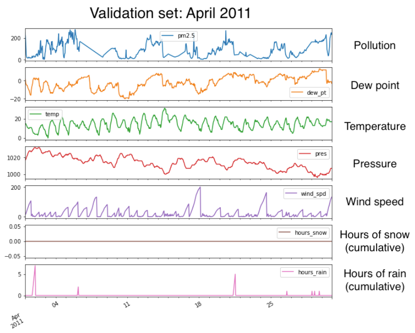
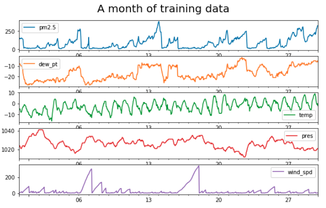
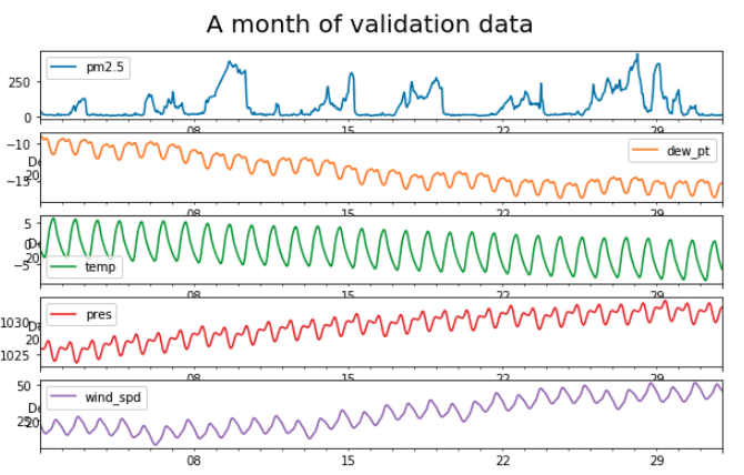
For my first experiments, I select a subset of the data spanning just over a year. I define a training set with data from January 2010 to March 2011, and a validation set with just April 2011. As you can see by the straight downward slope in the second week of April, I have to patch some holes in the pollution data using linear interpolation (first subplot below). There are no nulls in the weather features.

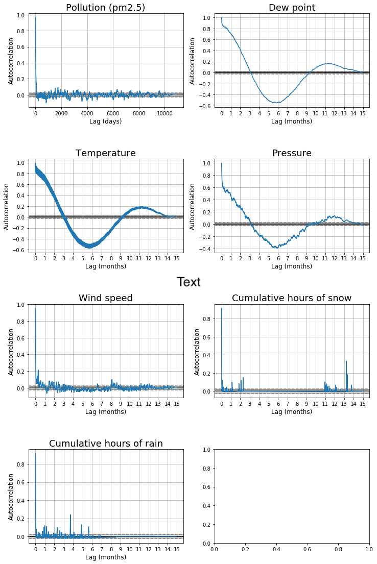
The plots below show how some of these features are markedly seasonal. In these autocorrelation plots, a variable with high seasonality will show sweeping curves far outside the narrow grey confidence intervals that hug the x-axis. Pollution doesn’t autocorrelate much beyond the last few hours, but temperature shows wide curves that stretch throughout the year.

As we’d expect, daily temperature correlates the most with the immediate past and with conditions one year ago. Dew point and pressure show a similar pattern, though you should note that the seasonality in temperature could show up in the other graphs if those weather variables are very temperature-dependent.

Capturing seasonality

There are many, many ways to capture the cyclic patterns in an autocorrelated dataset. The Statsmodels Time Series Analysis library, in particular, contains useful implementations of univariate autoregressive models (AR), vector autoregressive models (VAR), univariate autoregressive moving average models (ARMA), and non-linear models such as Markov switching dynamic regression and autoregression.

For this project, though, I use Prophet. It’s an open-source forecasting tool developed by Facebook that provides a particularly user-friendly interface for a variety of additive forecasting models. Prophet finds the seasonal trends in historical values of a variable, and uses them to build a linear regression model for predicting future values. It can even create multivariable regressive models, with the limitation that the extra regressors have to be known into the future. Data about time (holidays, days of the week, etc) are particularly easy to know about the future, and Prophet has built-in features for adding them.

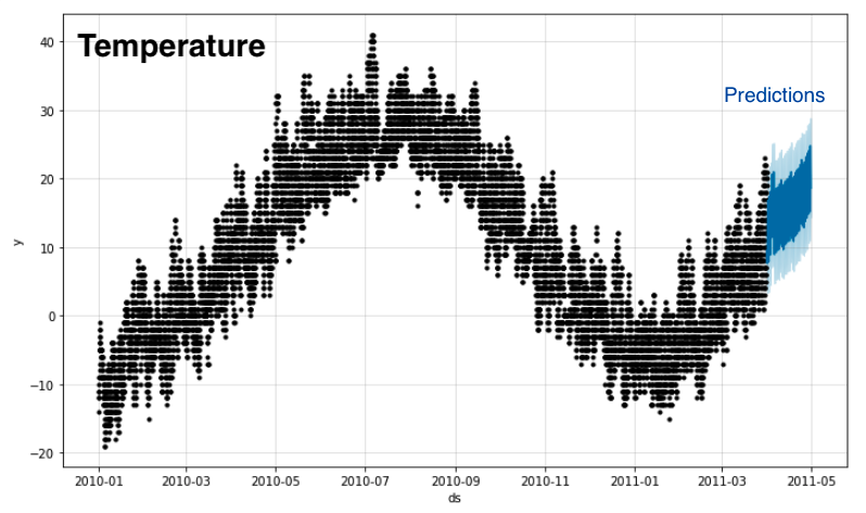
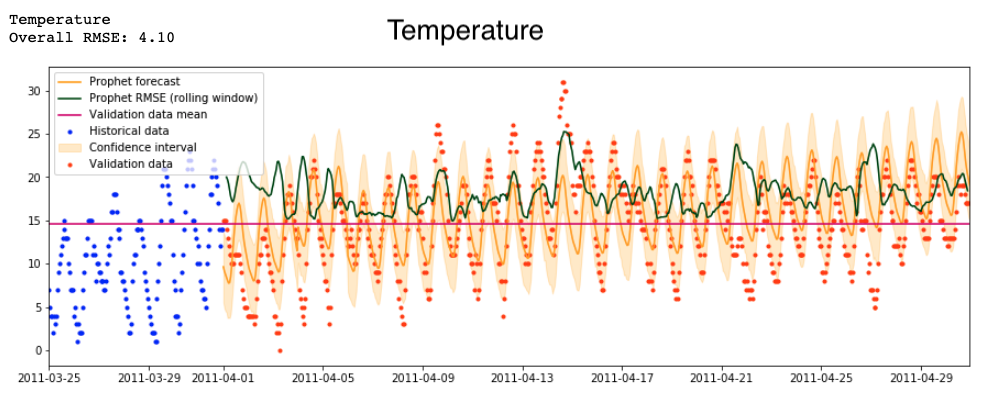
I feed Prophet historical temperature data and a list of Chinese holidays. This is what the model foretells:

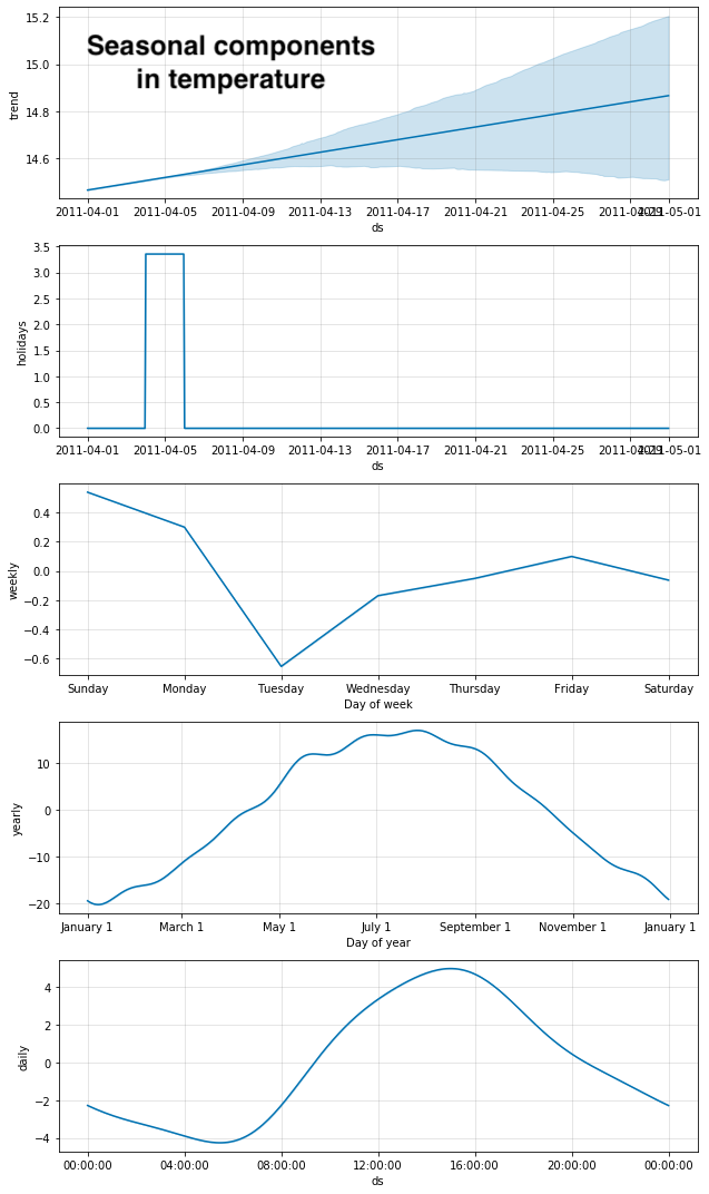
I particularly like how Prophet can show you a decomposed view of the seasonal trends that went into its predictions:

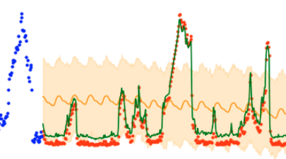
Here is a zoomed-in view of the tail end of the training data (blue) and validation data (red), along with Prophet’s forecast and confidence intervals (orange):

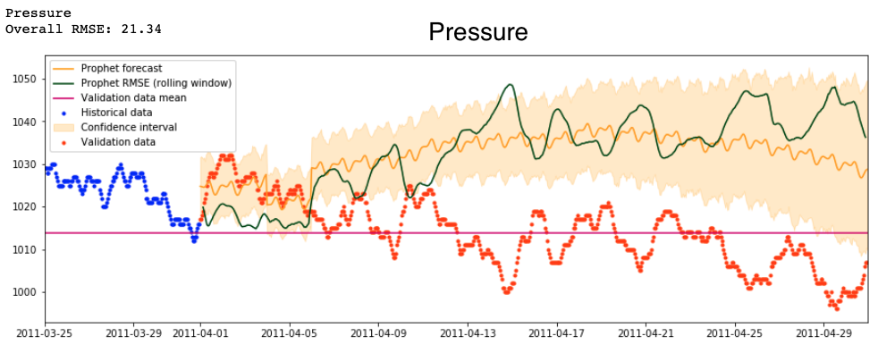
In contrast to the beautiful forecast for temperature above, Prophet is not able to handle the binary nature of my one-hot-encoded values for wind direction. It can only produce an uncertain floating-point prediction, so I drop wind direction from the dataset. I also drop the cumulative hours of rain and snow, since these values are almost always zero.

For most other variables, Prophet produces cyclical predictions that are relatively conservative—they hold a pattern with much more regular amplitude than we observe in real data.

Temperature bootstrapping?

At this point, I have an idea.

Prophet can add extra regressors to its univariate models, so long as their values are known into the future. Several of the weather variables are probably dependent on temperature—especially dew point, and probably pressure. Therefore, would it be possible to first forecast temperature into the future, and then use that prediction as an extra regressor for all the others?

Sadly, no.

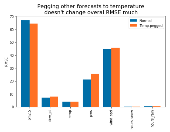
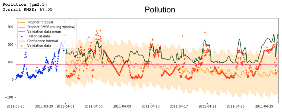
And so, in the end, this is the best prediction for pollution that Prophet can generate. It is cyclical, but otherwise far removed from the actual changes in pollution even at the very beginning of the forecast. This is a mild surprise, as I expected that its rolling-window RMSE (dark green line) would get higher as it moved further and further away from the last historical data point.

A neural network that sees only time

Several recent Kaggle competitions have seen great success (kaggle, arXiv) from a model that is almost too simple: a neural network with category embeddings and just two layers and no access to historical data points. It represents an approach entirely different from what Prophet does, and is nearly as easy to set up. I use the fast.ai library to make the model, which looks like this:

TabularModel(
  (embeds): ModuleList(
    (0): Embedding(3, 1)
    (1): Embedding(3, 1)
    (2): Embedding(13, 6)
    (3): Embedding(54, 26)
    (4): Embedding(32, 15)
    (5): Embedding(8, 3)
    (6): Embedding(366, 50)
    (7): Embedding(3, 1)
    (8): Embedding(3, 1)
    (9): Embedding(3, 1)
    (10): Embedding(3, 1)
    (11): Embedding(3, 1)
    (12): Embedding(3, 1)
    (13): Embedding(25, 12)
  )
  (emb_drop): Dropout(p=0.04, inplace=False)
  (bn_cont): BatchNorm1d(7, eps=1e-05, momentum=0.1, affine=True, track_running_stats=True)
  (layers): Sequential(
    (0): Linear(in_features=127, out_features=1000, bias=True)
    (1): ReLU(inplace=True)
    (2): BatchNorm1d(1000, eps=1e-05, momentum=0.1, affine=True, track_running_stats=True)
    (3): Dropout(p=0.001, inplace=False)
    (4): Linear(in_features=1000, out_features=500, bias=True)
    (5): ReLU(inplace=True)
    (6): BatchNorm1d(500, eps=1e-05, momentum=0.1, affine=True, track_running_stats=True)
    (7): Dropout(p=0.01, inplace=False)
    (8): Linear(in_features=500, out_features=1, bias=True)
  )
)

The original authors have commented very little on their exact choice of architecture and parameters. I try one variation with more layers and get the same results, so I decide not to optimize the model further for now.

I set up the neural net to see only two things: pollution and time. I use a helper function from fastai, add_datepart, to expand the Datetimeindex into a variety of time features for regression:

# df.columns
['pm2.5']

# df.columns after add_datepart
['pm2.5',
 'Year',
 'Month',
 'Week',
 'Day',
 'Dayofweek',
 'Dayofyear',
 'Is_month_end',
 'Is_month_start',
 'Is_quarter_end',
 'Is_quarter_start',
 'Is_year_end',
 'Is_year_start',
 'Hour',
 'Minute',
 'Second',
 'Elapsed']

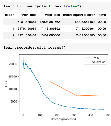
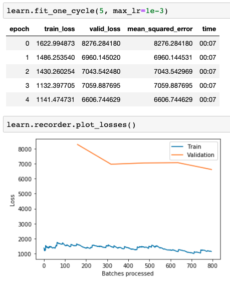
I fit the model for just a few epochs, until validation error bottoms out:

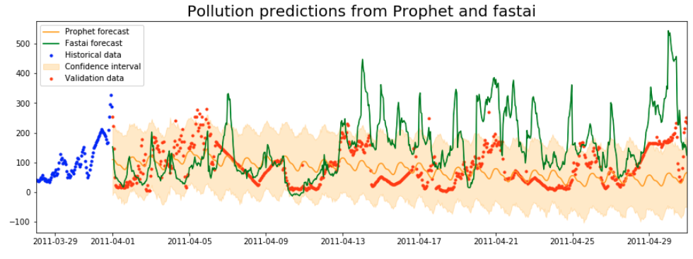
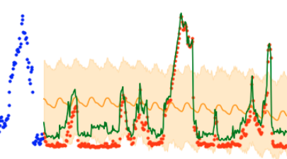
And finally, I compar its predictions with those from Prophet. The best validation loss I am able to get is 118.24 (that’s the overall RMSE for the month). This is clearly higher than my earlier losses of 67.05 and 64.46 from Prophet. As you can see below, the neural network predicts much more variation and has a much less clear cycle. It’s encouraging that the neural network actually seems to perform better for the first half of the month or so, issuing predictions that vary boldly in tandem with the actual data. Prophet issues relatively continuous predictions with much lower variability.

Adding awareness of weather

What I like about these neural net results is how much they reflect the seasonality of the pollution data even though the model is just a general-purpose pattern finder. Prophet is a bundle of models explicitly designed to find autocorrelative patterns, but it didn’t beat the net by that much.

A more fundamental problem is that Prophet, like other purpose-built models, is much more constrained by its design. I can’t find a way for Prophet to see the values of all the weather variables and use them for prediction, even though they’re very relevant. All that the system allows me to build is a univariate regression with an awareness of holidays.

A neural net, on the other hand, allows for creativity.

What if I give the net awareness of the current weather? Domain knowledge suggests that pollution should vary greatly with temperature and wind speed, so any patterns that the net sees in the weather data should make for a much stronger prediction of pollution.

Ah, but there is a catch.

Previously, my net was just training on time features, which are known arbitrarily far into the future. I know the values for current weather throughout the training data, but what about in the future?

I have weather data for the validation set, of course, but I don’t want the model to see it. In many examples I found around the internet, people predict one variable but still allow their model to see future values of all the others. Alternatively, their models predict one day into the future and then adjust based on what the day turned out to be like. In this project I want to tackle the much more interesting problem of predicting weather and pollution a full month into the unknown.

And so, this is where Prophet comes in. I can use it to forecast each of the weather features individually into the future, thereby populating the validation set with something that the neural net can use. This synthetic data doesn’t have nearly as much variability as the real stuff, but it beats using constant values or having to see into the future:

Adding awareness of history

Seeing the current weather (or predictions thereof) is definitely an improvement, but I think I can do even better. What if I give the net an explicit awareness of history? I bet the network could better pick out seasonal patterns if it could see what pollution was like a day, a month, and a year ago.

Pandas makes it possible to generate features offset by given amounts of time. I must do so very carefully, though, because offset features are dangerous. They can leak information from the future into the past.

Say that a validation set that starts on January 1st. On January 5th, we know what the weather was like a year, a month, and a week ago, but we don’t know what it was on January 1, 2, 3, or 4. Those dates are all still in the future.

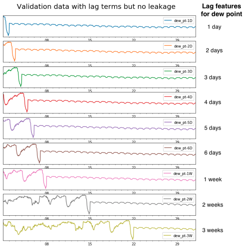
Time leakage is an important problem, but for offset features it can be prevented with just careful accounting. I generate offset features for pollution and weather, allowing the network to see back many days, weeks, months, and years back in time.

# Time offsets used for new features
days = [1,2,3,4,5,6]
weeks = [1,2,3]
months = [1,2,3,4,5,6]
years = [1,2,3]

And this is what one set of offset features looks like in the validation set:

Showtime!

And so, after all this feature engineering I’m finally ready to test the neural network. I switch to a larger train/test set covering almost 4 years, with November 2014 as the validation set. I bundle the data up into a fastai learner, and start training.

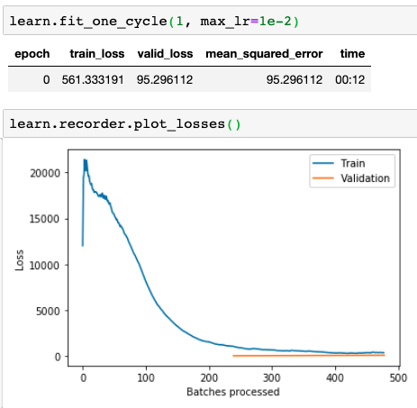
Huh, that’s funny.

Training error plumetts right away, in less than one epoch. By the time that the validation loss starts being measured halfway through, it’s already below the training loss.

I test this a few times, and in every case a single epoch brings the validation error all the way down. Why is it going so fast?

Also… hold on a second.

That validation error is equivalent to an overall RMSE of … 9.74?? That is fantastically better than the best validation loss I was able to get before, which was 118.24. The best that Prophet could produce was 64.46, back when I bootstrapped pollution predictions with temperature. This is amazing! In fact, it’s too amazing.

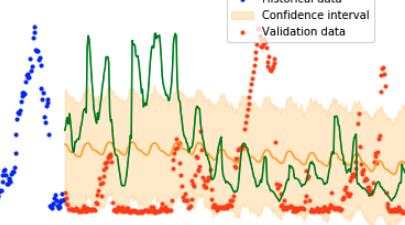
What does the validation data actually look like?

No. Fricken. Way.

That green prediction from the neural net absolutely hugs the data, all the way until the end of the month. Not only that, do you see how it even hugs the straight line in the data around November 21st? Those straight lines are interpolation artifacts caused by missing data, and should not be predictable based on the weather. Even worse, the model is just as perfect at the beginning of the month as at the very end, where all the net can work with is the predictions from Prophet.

These are the symptoms of severe data leakage. Somehow, the model is seeing the answers and spitting them back to me.

But how?!

Alright, so I’ve got data leakage. Let’s rule out possible causes.

If it’s a problem with the design of the offset features, despite my precautions, then this unnaturally perfect fit should degrade when I get rid of them. I trim the dataset and fit a new model.

It’s a bit less perfect. Could that have been it? But this is still much better than I’ve seen before. If the model is simply that good, then it should degrade gradually as I remove more variables. What happens when I get rid of temperature as well?

A bit less perfect again, but still suspiciously good. Alright, I’m getting rid of everything other than the dependent variable and the auto-generated time features.

Unbelievable! This is the same data that I’d used at the very beginning, how can it be so leaky?

I rewrite my fastai model a few times, in different ways, and eventually figure out the problem. Pollution is somehow not just being used as a dependent variable, but is bundled with all the features that the model is supposed to regress on. I switch to a different way of providing y-values to the learner, and at long last the model behaves the way it should.

Finally, some results

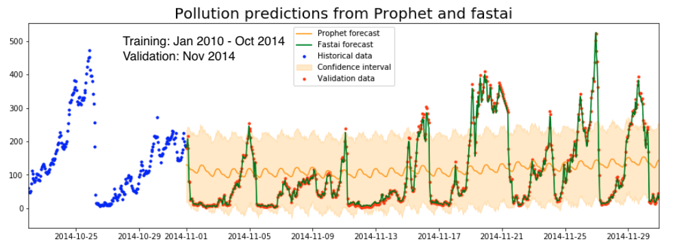
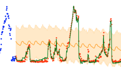
The full course of predictions looks like this:

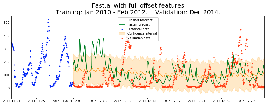
As you can see, the neural net still produces much greater, more natural variation than the regressive models inside Prophet. Though the predictions don’t align too much with the test data (the best RMSE here is about 86), the predictions have a more realistic shape and variance.

I expected that predictions would start out faithful and then degrade over the month, as more and more historical data is replaced with Prophet predictions. I don’t see that here. In fact, these predictions look no different to me than the ones that I produced earlier with just date information, without any offset historical features. This suggests that perhaps my intuition was wrong, and historical offsets don’t add that much information on top of what the model already knew based on time features.

Or perhaps I should just be using a more suitable neural network design. In a future project, I might explore recurrent neural networks designed to have an internal representation of history, such as LSTMs.

Lessons for the future

And so, dear reader, you now see how much of the real work in machine learning is not tuning the model itself, but rather designing the pipeline that feeds data to it. Neural networks are really creative in reducing their error metric. It is our job to anticipate when it could happen and to recognize when it has. Learn to adopt a security mindset, and learn to be suspicious of results that are too good to be true. Good luck out there.

You can find the full code for this project on GitHub.