I use the fast.ai deep learning library for one of its newest applications: predictive modeling on tabular data. I compare its performance against the incumbent best tool in the field, gradient boosting with XGBoost, as well as against various scikit-learn classifiers. Despite recent prominence on other tabular datasets, in this case fast.ai falls behind XGBoost and sklearn’s RandomForestClassifier.

Background

The Tanzanian Ministry of Water recently conducted a survey of tens of thousands of water pumps that had been installed around the country over the last several decades. The Ministry knew what kind of pumps existed, which organizations had installed them, and how the pumps were managed. The survey added one last important detail to the existing knowledge: did the pumps still work?

The Ministry’s data about the pumps and their status was collected into a dataset and organized into a competition by DrivenData, a platform that organizes data science competitions around problems with humanitarian impact. Predictive analytics on this dataset could allow the Ministry to know in advance which pumps are most likely to be non-functional, so that they can triage their repair efforts. It’s hard to find much simpler examples of how a good predictive model can directly save time and money.

You can find the full notebook for this analysis on the Github repo.

Blue means ‘working’, gold means ‘broken’, and green means ‘needs repair’.

Extensive data cleaning and feature engineering were needed to process the data for the nearly 60,000 water pumps in this dataset. Many of the categorical features had high cardinality (100s - 1000s of uniquevalues), and many features consisted of manually typed strings with lots of user errors. My data exploration involved significant amounts of RegEx to spot input errors and collapse redundant categories.

Tabular Deep Learning with fast.ai

The tabular functionality in fast.ai combines training, validation, and (optionally) testing data into a single TabularDataBunch object. This structure makes it possible to tune pre-processing steps on the training data and then apply them equally to the validation and test data. Thus, with fast.ai the process of normalizing, inputing missing values, and determining the categories for each categorical variable is largely automated. More interestingly, as we’ll see below, this processed data can be used to fit models from other libraries.

# 'train' is all the training data, including the dependent variable. 
# It was cleaned in earlier steps but still contains nulls and hasn't 
# been normalized yet. 'dep_var' is the name of the dependent variable;
#  'cat_names', and 'cont_names' are lists of the categorical and 
# continuous features, respectively. 'train' will be used as the 
# source of both training and validation data. 


# Transformations to be applied later
procs = [FillMissing, Categorify, Normalize] 

# Test data
test = TabularList.from_df(X_test, 
                           cat_names=cat_names, 
                           cont_names=cont_names)

# Creates the overall TabularDataBunch ('data'), which includes 
# training data (the first 50,000 rows in 'train'), validation 
# data (the last 9,400 rows in 'train'), and test data 
# (the TabularList 'test').
data = (TabularList.from_df(train, 
                            cat_names=cat_names, 
                            cont_names=cont_names, 
                            procs=procs)
                    .split_by_idx(list(range(50000,59400)))
                    .label_from_df(cols=dep_var)
                    .add_test(test)
                    .databunch())

Fast.ai creates embeddings for all the categorical variables, grouping them so that the similarities between category members can be exploited. I set the embeddings to half the size of each variable’s cardinality, up to a max of 50. This is a rule of thumb presented in the fast.ai courses, which overrides the library’s default embedding size.

# Creates dictionary of embedding sizes for the categorical features
categories = X_train_processed[cat_names].nunique().keys().to_list()
cardinalities = X_train_processed[cat_names].nunique().values
emb_szs = {cat: min(50, card//2) for cat, card in zip(categories, cardinalities)}
emb_szs

I created a tabular learner with relatively large layers, modeled after the architecture that was used to earn the third place in the Rossman Kaggle competition. I regularize the model using dropouts for both layers (0.001, 0.01) and embeddings (0.04).

# Creates the tabular leraner
learn = tabular_learner(data, emb_szs=emb_szs, layers=[1000,500], 
                        ps=[0.001,0.01], metrics=accuracy, emb_drop=0.04)

# Prints out the model structure.
learn.model

Note how there is one embedding for each of the 23 categorical features.

TabularModel(
  (embeds): ModuleList(
    (0): Embedding(143, 50)
    (1): Embedding(126, 50)
    (2): Embedding(36, 18)
    (3): Embedding(10, 4)
    (4): Embedding(61, 30)
    (5): Embedding(22, 10)
    (6): Embedding(18, 9)
    (7): Embedding(124, 50)
    (8): Embedding(309, 50)
    (9): Embedding(3, 1)
    (10): Embedding(12, 6)
    (11): Embedding(87, 43)
    (12): Embedding(3, 1)
    (13): Embedding(16, 8)
    (14): Embedding(12, 6)
    (15): Embedding(5, 2)
    (16): Embedding(7, 3)
    (17): Embedding(7, 3)
    (18): Embedding(5, 2)
    (19): Embedding(10, 5)
    (20): Embedding(3, 1)
    (21): Embedding(7, 3)
    (22): Embedding(3, 1)
  )
  (emb_drop): Dropout(p=0.04)
  (bn_cont): BatchNorm1d(9, eps=1e-05, momentum=0.1, affine=True, track_running_stats=True)
  (layers): Sequential(
    (0): Linear(in_features=365, out_features=1000, bias=True)
    (1): ReLU(inplace)
    (2): BatchNorm1d(1000, eps=1e-05, momentum=0.1, affine=True, track_running_stats=True)
    (3): Dropout(p=0.001)
    (4): Linear(in_features=1000, out_features=500, bias=True)
    (5): ReLU(inplace)
    (6): BatchNorm1d(500, eps=1e-05, momentum=0.1, affine=True, track_running_stats=True)
    (7): Dropout(p=0.01)
    (8): Linear(in_features=500, out_features=3, bias=True)
  )
)

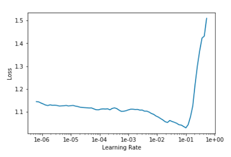
The lr_find() function in fast.ai allows one to see the loss that different learning rates would cause. The ideal learning rate for fitting this model is located around the middle of the steepest downward slope before the graph bottoms out (about 1e-02).

learn.lr_find()
learn.recorder.plot()

The built-in fit_one_cycle() method can fit the model with a varying learning rate that starts low, ramps up to the maximum, and then goes low again. This learning rate annealing is known to work much better than just choosing a single rate. I fit the model for a few epochs.

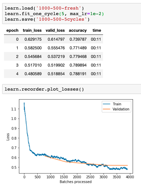
And then again for a couple more, inching ahead so long as the validation loss keeps falling.

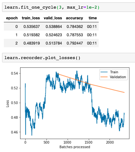
By saving my model after every couple of fitting epochs, I can keep going until it starts overfitting (when the validation loss starts creeping up again). I did that a couple of times, then reverted to the last batch of fitting that had still improved the model. In the end, I was able to get an accuracy of 79.2%, which fast.ai automatically calculates on the validation set in the same TabularDataBunch.

Other models

Regardless of the actual deep learning it is designed to do, the fast.ai library is useful for pre-processing data for all sorts of models. It normalizes, creates categories, and fills in missing values. I wrote a custom function to retrieve that data from the TabularDataBunch object, and used an ordinal encoder to encode by the categories present in the training dataset.

from category_encoders.binary import BinaryEncoder
def get_proc_df(tdb, cat_names, cont_names):
    """Get processed xs and ys from a TabularDataBunch with training and validation
     datasets.
       :param tdb: A TabularDataBunch. 
       :param cat_names: Array of strings for the categorical variables
       :param cont_names: Array of strings for the continuous variables
       :returns: A tuple of `(X_train, X_valid, y_train, y_valid)` 
        where `X_` items are a pandas `DataFrames` and `y` items are numpy arrays.
    """
    
    def list_to_df(tll):
        """
        Takes a tabular list (the training or validation data in this 
        TabularDataBunch) and returns its items as a pandas DataFrame.
        """
        x_vals = np.concatenate([tll.x.codes, tll.x.conts], axis=1)
        x_cols = tll.x.cat_names + tll.x.cont_names
        x_df = pd.DataFrame(data=x_vals, columns=x_cols)[
                [c for c in tll.inner_df.columns if c in x_cols] ] # Retain order
        y_vals = np.array([i.obj for i in tll.y])
        return x_df, y_vals
    
    X_train, y_train = list_to_df(tdb.train_ds)
    X_valid, y_valid = list_to_df(tdb.valid_ds)
    
    # Binary encode the categorical variables, according to their values in 
    # the training dataset
    encoder = BinaryEncoder(cols=cat_names)
    X_train = encoder.fit_transform(X_train)
    X_valid = encoder.transform(X_valid)
    
    return X_train, X_valid, y_train, y_valid

X_train, X_valid, y_train, y_valid = get_proc_df(data, cat_names, cont_names)

I then put these processed datasets through a variety of classifiers, each instantiated with the default values.

from sklearn.ensemble import RandomForestClassifier
from sklearn.linear_model import RidgeClassifier, LogisticRegression
from sklearn.discriminant_analysis import LinearDiscriminantAnalysis
from sklearn.naive_bayes import GaussianNB, BernoulliNB
from sklearn.tree import DecisionTreeClassifier
from sklearn.svm import LinearSVC
from sklearn.metrics import log_loss
from sklearn.metrics import accuracy_score
from xgboost import XGBClassifier

classifiers = [
    RandomForestClassifier(),
    LogisticRegression(solver='lbfgs', multi_class='ovr', max_iter=500),
    LinearDiscriminantAnalysis(),
    GaussianNB(),
    BernoulliNB(),
    DecisionTreeClassifier(),
    XGBClassifier(objective = 'multi:softmax', booster = 'gbtree', 
                     nrounds = 'min.error.idx', num_class = 3, 
                     maximize = False, eval_metric = 'logloss', eta = .1,
                     max_depth = 14, colsample_bytree = .4, n_jobs=-1)
]

results = pd.DataFrame(columns=["Classifier", "Accuracy"])

for clf in classifiers:
    name = clf.__class__.__name__
    clf.fit(X_train, y_train)
    acc = accuracy_score(y_valid, clf.predict(X_valid))
    
    log_entry = pd.DataFrame([[name, acc*100]], columns=["Classifier", "Accuracy"])
    results = results.append(log_entry)

results = results.append(pd.DataFrame([['fast.ai', 79.2]], columns=["Classifier", "Accuracy"]))
results = results.sort_values('Accuracy', ascending=False)

fig, ax = plt.subplots(1,1, figsize=(6,5))

ax.barh(results['Classifier'], results['Accuracy'], color="b")
ax.tick_params(axis="y", labelsize=14)
ax.set_xlabel('Accuracy %', fontsize=14)
ax.set_title('Classifier Accuracy', fontsize=20);

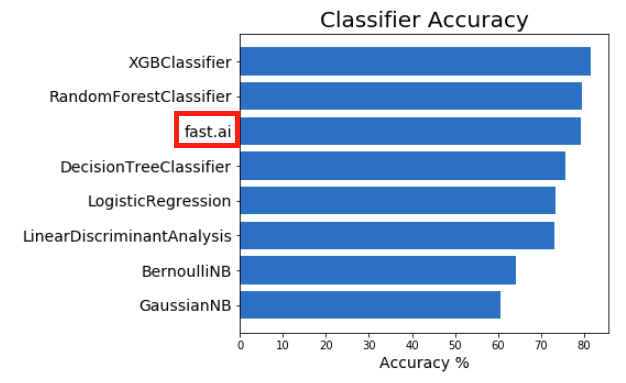
And so, at least for this dataset, XGBoost and RandomForestClassifier beat fast.ai, in the former case by a significant margin. All this goes to show the importance of testing and tuning a few different methods.

Despite the conventional results in this particular experiment, deep learning is increasingly beig used for tabular datasets and can generate great results with relatively minimal feature engineering. Embeddings make it possible to group together similar values in even highly-cardinal categorical features. Proper use of dropout, weight decay, and other regularization methods ensure that overfitting remains in check even for huge models with lots of parameters. The applications are as varied as tabular data itself, so it’ll be interesting to see how different approaches compare to each other in the future.